Last Month I had the opportunity to design a content recommendation system and I decided to go with BigData due to the scope of the problem. After successfully implementing it and running it on a training dataset consisting of around 2.8 million ratings given by 73,000 people spread across 1600 movies, I’m about to share my views on the idea as a whole.
This is going to be a big article compared to my usual ones as I’ll be touching upon all the options I had and why I selected the ones I used for my implementation. The below jump lists can be used to go to a specific section directly.
- Let’s talk Optimizations !!
- Reducing the data flow
I would go as far as to say that my implementation is a naive version of the Collaborative filtering algorithm as it only factors the user likes. So although this algorithm is not going to dethrone the best of the best used by the industry stalwarts like Google or Netflix, it doesn’t need to. My main aim here was to play around with the advance MapReduce concepts and use it for some challenging use cases like graph creation and processing. So without further ado, let’s get started !!
You can find the entire project hosted at my github repo here –> https://github.com/kitark06/recommender
The Training Dataset I used belongs to the Digital Equipment Corporation. You can check that link for the schema definition which will be needed to parse the dataset. The actual dataset can be downloaded from this link & consists of 2 files which are of particular interest.
- The Movies.txt which contains 1628 different movie metadata like the MovieName and MovieId and is sorted by movieID.
- The Vote.txt which is the most important file and contains 2811983 mappings of the userID and the MovieId which he has liked.
This dataset will be fed into the MapReduce code which will then allow us to get the recommended movies arranged in a most liked to least liked movies for any given movie.
The Overview.. featuring Collaborative Filtering
The algorithm that I have implemented factors in the similarity between the user likes to calculate its recommendations and is a type of the Collaborative filtering approach which roughly means something along the lines of
Given two persons “A” and “B” who share similar tastes, B will supposedly like and prefer a movie/song which is also liked by A .. as compared to some content liked by a random person.
It involves creation of a graph/mesh-like interconnected representation of all the content where
- Each Vertex/Node of the graph is a unique content which in this example is a Movie.
- The Edges of the graph represent the similarity between the Nodes.
- Weights(numerical value) are assigned to all the edges, which is equal to the number of users liking both Movie1 and Movie2.
Although the example I which have used below shows the data in a sorted and ordered manner, this is simply for ease of explanation. In the actual input, the data will NOT be sorted and it doesn’t need to be. Due to the nature of MapReduce, the algorithm works irrespective of the input order.
The graph is the result of the processing the input and contains the following information.
- 4 movies say A, B, C & D (liked by 5 unique users).
- There are for example, 3 Users who have liked both movies A & B while only one user who has liked A & D
- So if a new User likes movie A , the recommendations will be B,C,D in that order due to their weights with A being 3, 2 & 1 respectively.

The Algorithm.. designing around MapReduce
The implementation of this algorithm in Core Java would make the coding very simple but the resulting application wouldn’t be feasible as the memory requirements of such a system would be immense for large scale input since the resulting graph would have to fit into memory for almost the entire duration of the program execution. Well technically the data could be serialized and written to disk, but that’s only possible after the graph is created. Also the entire Graph would have to be deserialized back to memory before the it can be queried.
Although the representation of a Graph in MapReduce is very challenging because of the File based nature of Hadoop, adopting this paradigm allows us to circumvent any memory limitations imposed by a traditional approach. This sole reason justifies the additional programming efforts required to design our application around the strengths of MapReduce.
Consider the input to the program is generated by a system which logs the UserID and MovieID to a text file when the user likes a movie. Thus the input is unordered and randomly sorted. So the first stage of input is a string which has a UserID and MovieID separated by Tab char ‘t’
Phase One – Parsing The Input.
Here the aim of the program is to group all the MovieIDs liked by a single user, which is done iteratively for each user. This falls in line with the use case of MapReduce where
- The Mapper will get the below lines of String as input and will emit a key/value pair. The output of phase 1 Mapper will go as input to the Reducer.
- Reducer will group all the values for each key, which here is to group all of the MovieIDs liked by each user.
(Reducer output values are unsorted/randomly ordered because although the input keys which it receives are guaranteed to be sorted, the values aren’t )
| Input (UserID –> MovieID) | Output (UserID –> Set<MovieID> ) |
|---|---|
| u2 –> B u5 –> C u1 –> A u3 –> A u4 –> A u2 –> A u1 –> B u3 –> B u4 –> C u5 –> A u1 –> D |
u1 –> [B,D,A] u2 –> [B,A] u3 –> [A,B] u4 –> [C,A] u5 –> [A,C] |
Phase Two – Preparing The Graph.
This part of the program consists of a second MapReduce job which generates Permutations of the above groups. This helps to calculate the graph edge weights.
- The Mapper will generate all the possible Bi-gram (pair of 2) Permutations of the given comma separated MovieIDs as the Key and the value as integer one.
So for eg :: A,B,D will be converted to AB , BA , BD , DB , AD & DA - The Reducer will simply aggregate the count of all the values for each key and will emit a key and total count. I.e The key will be the graph edge and the count will be the total weight.
In the output of this phase, the UserID info is practically discarded as it’s irrelevant to us now that all the needed user-likes info is extracted & contained within the groups which are formed.
| Mapper Input (UserID –> Set<MovieID>) |
Mapper Output (MovieID1,MovieID2 –> One ) |
Reducer Output (MovieID1,MovieID2 –> No of people who liked M1 and M2) |
|---|---|---|
| u1 –> [B,D,A] u2 –> [B,A] u3 –> [A,B] u4 –> [C,A] u5 –> [A,C] |
BD –> 1 DB –> 1 DA –> 1 AD –> 1 BA –> 1 AB –> 1 BA –> 1 AB –> 1 AB –> 1 BA –> 1 CA –> 1 AC –> 1 AC –> 1 CA –> 1 |
AB –> 3 BA –> 3 BD –> 1 DB –> 1 AD –> 1 DA –> 1 AC –> 2 CA –> 2 |
Readers familiar with MapReduce will draw parallels between this approach and the classic WordCounter problem & rightfully so !! In my first article which i wrote about BigData setup, I went in detail about the setup and concluded that post by executing the WordCounter which is considered as the Hello World of MapReduce. You can check that article here –> Hadoop on Windows
With the reducer’s final output in front of us, it’s easy to visualize the Graph which is an abstract representation of the diagram shown below.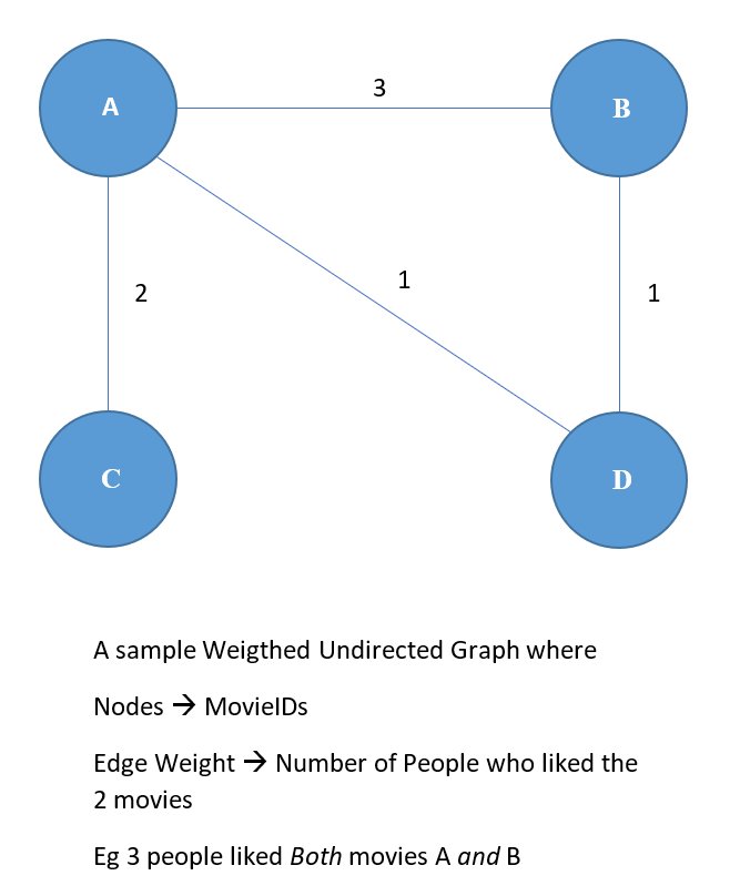
Looking at the output of the reducer,
- AB –> 3 represents that the Edge between A and B is 3.. similarly
- AC –> 2 represents that the Edge between A and C is 2
The contents of this file are stored in a text file on disk atop the H.D.F.S – Hadoop’s distributed file system. Thus there is very little memory utilization for creating the graph as most of the time, the graph spends its life in text files and the entire Graph is never loaded into memory all at once.
Phase Three – Generating the Recommendations (Querying the Graph).
The final phase of the program is responsible for generating the Recommendations. In this last MapReduce job, for each Movie M1 we will get a list of all the other movies and display it in descending order based on the number of users who have liked that other movies respectively. A descending Secondary sort is used to achieve this.
Now let me make this clear, though the input which a reducer gets from mapper is sorted, it’s only sorted by keys. We want the keys to have values which are Reverse sorted. Hence the need for Secondary Sorting.
- The Mapper.
Takes in the graph as input and will emit a Key_Composite which is a custom Implementation of the writable interface.
This Composite key will have both the Key as well as the Value (eg A [B, 3]). - The Partitioner.
will use the Key_Composite.Key (eg A [B, 3]) will be used for partitioning the data.
What this means is that keys with the same source node will go to the same reducer. So {A [B, 3]} , {A [D, 1]} & {A [C, 2]} will go to the same reducer. - The DescendingSortComparator
This stage is responsible for the actual reverse sorting based on the edge weights. The Key_Composite.Value (eg A [B, 3]) is used here.
So {A [B, 3]} , {A [D, 1]} & {A [C, 2]} becomes {A [B, 3]} , {A [C, 2]} & {A [D, 1]} - The ReduceGroupComparator
Responsible for grouping and then sending all the CompositeKeys to the reducer.
So {A [B, 3]} , {A [C, 2]} & {A [D, 1]} becomes A <[B, 3], [C, 2], [D, 1]> - The Reducer
Hardly does any work as all the heavy lifting computation is done before the Reducer gets its input.
The Reducer merely writes what it gets as input to a text file.
| Mapper Input (MovieID1,MovieID2 –> No of people who liked M1 and M2) |
Mapper Output (SourceNode –> [DestinationNode, Weight]) |
Reducer Output (MovieID–> Recommended Movies for that MovieID) |
|---|---|---|
| AB –> 3 BA –> 3 BD –> 1 DB –> 1 AD –> 1 DA –> 1 AC –> 2 CA –> 2 |
{A [B, 3]} –> [B, 3] {B [A, 3]} –> [A, 3] {B [D, 1]} –> [D, 1] {D [B, 1]} –> [B, 1] {A [D, 1]} –> [D, 1] {D [A, 1]} –> [A, 1] {A [C, 2]} –> [C, 2] {C [A, 2]} –> [A, 2] |
A –> [B 3], [C 2], [D 1] B –> [A 3], [D 1] C –> [A 2] D –> [B 1], [A 1] |
And with this, the chain of the 3 phases of MapReduce jobs is complete and the recommendations for each of the movies has been generated. This file is obviously not intended to be human readable and as the number of movies increases it’ll soon become incomprehensible. But that’s perfectly alright as this file will go as input to the part of the program which is responsible for the view generation.
So if we consider a Service Oriented Architecture, then our application can be hosted as a service and for any given movie, a view generator will ask for recommendations and accordingly will sort them based on most liked to least liked movies. For the scope of this article, I’ll stop here at the recommendation service and won’t go ahead into the view generation aspects. What I will focus upon next are optimizations..
Let’s talk Optimizations !!
Before I talk about the various ways in which one can optimize MR jobs, let’s first have a look at the data flow between the Mapper and the Reducer in a typical MapReduce workflow.
InputSplits are calculated for each file in the input directory and for each split, a Map task is created and executed. In HDFS, each file is replicated thrice (by default). So in a big cluster, MapTasks are tried to be executed on one of the 3 node which has the InputSplit. This is done to reduce data flow, which is in line with the MapReduce paradigm “Move Code to Data & not vice versa“.
The most important things to consider here are
- Although the Map tasks are tried to be scheduled on the same node which has the data (Data locality), Reduce tasks are not data local.
- The output of MapTask is written onto local disk of the node which executed the MapTask ; and not on HDFS. This output is sent to a reducer.
- Reducer Input Data is transferred across the network
This is done because on a large cluster the mappers and reducers could be and most likely would be running on separate physical machines. So data is serialized and sent across the network from the node which ran the map task, to the node which runs the reduce task for that particular key/partition.
All these shuffling and transfer phases I just listed above are extremely slow as they are primarily disk-bound and network-bound operations as compared to data which is processed in-memory.

Reducing the data flow
Now that we have an idea about how data moves from a Mapper to Reducer, it’s easy to see why reducing the data flow is perhaps the most significant optimization that can be done which impacts performance big time. This reduction can be achieved by myriad ways, with the most significant ones being listed below
- Changing the Algorithm
- Compressing just Map output or whole Job output.
- Using Combiners.
1. Changing the algorithm.
The most obvious, yet ironically the most oblivious and overlooked, changing the algorithm is akin to performing optimization at a grass root level. Now although there isn’t a “one size fits all approach” some ideas can be reused and modified to suit the context of your application. Let me give you a practical demo of the kind of algorithmic data reduction which can be performed.
Optimizing Phase One.
OLD output
| Input (UserID –> MovieID) | Output (UserID –> Set<MovieID> ) |
|---|---|
| u2 –> B u5 –> C u1 –> A u3 –> A u4 –> A u2 –> A u1 –> B u3 –> B u4 –> C u5 –> A u1 –> D |
u1 –> [B,D,A] u2 –> [B,A] u3 –> [A,B] u4 –> [C,A] u5 –> [A,C] |
Optimized — The MovieIDs in the reducer’s output are sorted in ascending order using secondary sort
| Input (UserID –> MovieID) | Output (UserID –> Set<MovieID> ) |
|---|---|
| u2 –> B u5 –> C u1 –> A u3 –> A u4 –> A u2 –> A u1 –> B u3 –> B u4 –> C u5 –> A u1 –> D |
u1 –> [A,B,D] u2 –> [A,B] u3 –> [A,B] u4 –> [A,C] u5 –> [A,C] |
Optimizing Phase Two.
Instead of generating permutations, the optimized Mapper will only generate all the possible Bi-gram (pair of 2) combinations of the given comma separated MovieIDs as the Key and the value as integer one.
So for eg :: A,B,D will be converted to AB , BD & AD
OLD output
| Mapper Input (UserID –> Set<MovieID>) |
Mapper Output (MovieID1,MovieID2 –> One ) |
Reducer Output (MovieID1,MovieID2 –> No of people who liked M1 and M2) |
| u1 –> [B,D,A] u2 –> [B,A] u3 –> [A,B] u4 –> [C,A] u5 –> [A,C] |
BD –> 1 DB –> 1 DA –> 1 AD –> 1 BA –> 1 AB –> 1 BA –> 1 AB –> 1 AB –> 1 BA –> 1 CA –> 1 AC –> 1 AC –> 1 CA –> 1 |
AB –> 3 BA –> 3 BD –> 1 DB –> 1 AD –> 1 DA –> 1 AC –> 2 CA –> 2 |
Optimized — As you can see, we have effectively halved the data which goes from the mapper to reducer & also the reducer output.
| Mapper Input (UserID –> Set<MovieID>) |
Mapper Output (MovieID1,MovieID2 –> One ) |
Reducer Output (MovieID1,MovieID2 –> No of people who liked M1 and M2) |
| u1 –> [A,B,D] u2 –> [A,B] u3 –> [A,B] u4 –> [A,C] u5 –> [A,C] |
AB –> 1 BD –> 1 AD –> 1 AB –> 1 AB –> 1 AC –> 1 AC –> 1 |
AB –> 3 BD –> 1 AD –> 1 AC –> 2 |
Importance of secondary sort.
If the Input to the mappers is not sorted on the Values, the mapper would get input with randomly sorted values which leads to the problem shown below where the total count in the reducer is split across the keys because AB and BA are considered as 2 separate keys and thus the resulting count mismatch.
| Mapper Input (Unsorted Values) | Mapper Output | Incorrect Reducer Output | Expected Reducer Output |
| u1 –> [D,A,B] u2 –> [A,B] u3 –> [B,A] |
DA –> 1 AB –> 1 DB –> 1 AB –> 1 BA –> 1 |
AB –> 2 BA –> 1 DA –> 1 DB –> 1 |
AB –> 3 AD –> 1 BD –> 1 |
Optimizing Phase Three.
The Mapper of Phase 3 is responsible for generating Permutations and AB is converted to AB and BA
OLD mapper input
| Mapper Input (MovieID1,MovieID2 –> No of people who liked M1 and M2) |
Mapper Output (SourceNode –> [DestinationNode, Weight]) |
Reducer Output (MovieID–> Recommended Movies for that MovieID) |
| AB –> 3 BA –> 3 BD –> 1 DB –> 1 AD –> 1 DA –> 1 AC –> 2 CA –> 2 |
{A [B, 3]} –> [B, 3] {B [A, 3]} –> [A, 3] {B [D, 1]} –> [D, 1] {D [B, 1]} –> [B, 1] {A [D, 1]} –> [D, 1] {D [A, 1]} –> [A, 1] {A [C, 2]} –> [C, 2] {C [A, 2]} –> [A, 2] |
A –> [B 3], [C 2], [D 1] B –> [A 3], [D 1] C –> [A 2] D –> [B 1], [A 1] |
Optimized — Mapper now gets 50% of the input in the Map phase from the optimized Phase 2 Reducer output.
| Mapper Input (MovieID1,MovieID2 –> No of people who liked M1 and M2) |
Mapper Output (SourceNode –> [DestinationNode, Weight]) |
Reducer Output (MovieID–> Recommended Movies for that MovieID) |
| AB –> 3 BD –> 1 AD –> 1 AC –> 2 |
{A [B, 3]} –> [B, 3] {B [A, 3]} –> [A, 3] {B [D, 1]} –> [D, 1] {D [B, 1]} –> [B, 1] {A [D, 1]} –> [D, 1] {D [A, 1]} –> [A, 1] {A [C, 2]} –> [C, 2] {C [A, 2]} –> [A, 2] |
A –> [B 3], [C 2], [D 1] B –> [A 3], [D 1] C –> [A 2] D –> [B 1], [A 1] |
Impact of Changing the algorithm.
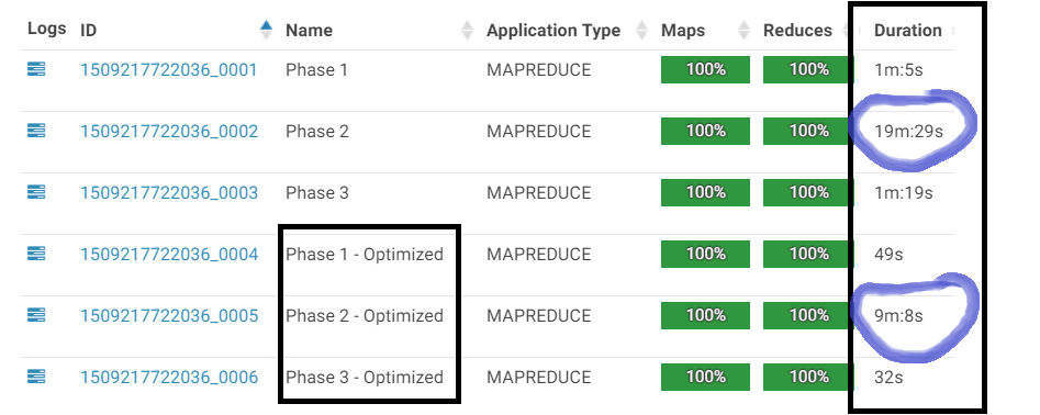
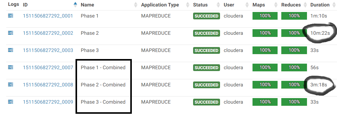
- In the Optimized Phase 2 we cut the data by half, which was produced and consumed by the mapper & reducer respectively. This 50% reduction in data throughput is reflected by a proportional reduction in runtime. 19 minutes –> 9 minutes
- We see a similar observation in the Optimized Phase 3 as the mapper just gets half the input and thus less data is moved across the node. The result is again a reduction of more than 50% in the runtime required for completion. 1 Minute –> 30 seconds
2. Enabling Compression
Compression is the easiest way of increasing throughput by compressing the data before it is shuffled and written on the disk &/or sent across the network. We just saw how data moves in a MapReduce workflow and from that it’s easy to see that compression boosts the speed at multiple stages like :
- Less data from the mapper output is written on the disk. This is called Intermediate data compression.
- Less data is sent to the reducer across the network.
- Less data is generated from the reducer’s output which gets written on the HDFS. This is called Job output compression.
It’s so easy and rewarding that instead of pondering “When should I use compression ?” the correct question to ask is “When should I NOT use compression ?” The answer to which is that we don’t when the file we’re dealing with is using a format which is natively compressed like MP3 file or JPEG. And in all the other scenarios enable compression.
To use compression, all we have to do is specify the stage to compress along with the compression codec. Choice of the codec is influenced by parameters like the
- Speed
- Compression ratio and
- Whether the compressed files are required to splittable. (only Files stored on HDFS needs to be spllitable)
Splittability means whether a particular file can be processed in parallel or not. NOT to be confused with the HDFS InputfileSplits.
Let me explain it with an example. Say we upload a 1280 mb file and the splitSize is 128mb, then file will be sharded and split into 10 * 128mb chunks and for a splittable file 10 MapTasks will be created and scheduled for execution. Thus, if the file is splittable, then hypothetically the 10 MapTasks can be executed in parallel by 10 separate mappers. If the file is not splittable, then only a single MapTask is created for a single file regardless of its file size and/or chunks and a single Mapper will end up processing the single MapTask which comprises the entire file of 10 chunks.
This is catastrophic as not only are we losing out on the parallelism offered by Hadoop, but the 10 chunks making up the 1280 mb file (which are most likely spread across the cluster) will have to be transferred across the network and fed to the single mapper process.
Intermediate data compression which happens between the mapper and reducer is controlled by
configuration.set("mapreduce.map.output.compress", "true")&- Codec is set by
configuration.set("mapreduce.map.output.compress.codec", "org.apache.hadoop.io.compress.SnappyCodec")
Snappy is used here as it provides a balanced and speedy compression/decompression & albeit not splittable, it’s not an issue as the Mapper output files are never stored on HDFS and hence splittability is not a concern.
Job output compression which compresses the job outputs which are stored on HDFS are controlled by
configuration.set("mapreduce.output.fileoutputformat.compress", "true")configuration.set("mapreduce.output.fileoutputformat.compress.type", "BLOCK")configuration.set("mapreduce.output.fileoutputformat.compress.codec", "org.apache.hadoop.io.compress.BZip2Codec")
Bzip2 is used here to get the benefits of compression along with splittability as well since the output of reducer is written onto HDFS. BLOCK compression level compresses multiple blocks of the output file (which are stored as SequenceFiles).
Impact of Enabling Compression.
We can verify that the compression is enabled & working by checking out the Map Output Bytes and Map Output Materialized Bytes counter. By simply noticing reduction in runtime here, the impact of compression seems immense.
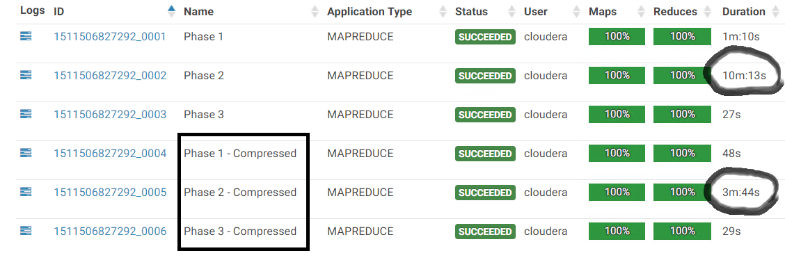
But its the reduction in network traffic which is significant. 2758 MB to 159 MB. That’s an astounding reduction in the amount of data written and subsequently carried across the network to the reducers.

3. Using The Combiner
The Combiner can be thought of like a MapSide Pre-Reduce stage operation which the Hadoop framework executes when the number of map partitions increases or is equal to 3 under default behavior conditions. Hence the execution of Combiner is not guaranteed.
When the framework does indeed execute the combiner, the amount of data is combined / reduced in the Mapper and hence less data is sent to the reducer as a result. The Combiner has the same method signature as the reducer and although the framework allows us to specify separate implementations for each, in most cases they both share the same implementation class.
We can see a similar trend here as reducing the amount of data directly results in a significant speed bump.
4. Re-using writables
The Hadoop FileSystem Writable objects are specifically designed for better serialization and most of them are analogues to Java data types like Text (String) LongWritable (Long) etc. The framework delivers the input to both the map and reduce functions in the writable datatype and the output also has to be one of the writables which the user can decide.
One naive mistake which amateurs make here is that they create a new Writable object inside the Map/Reduce function and use that to write the values to the Context (Output). This leads to a massive amount of very short lived objects created and destroyed over the course of a MapReduce job and leads to a very high GarbageCollection cycle.
The simple way to avoid this would be to Create the Writable Objects once at Instance level, and simply re-use those objects by changing their values, instead of creating them anew.
The Conclusion.
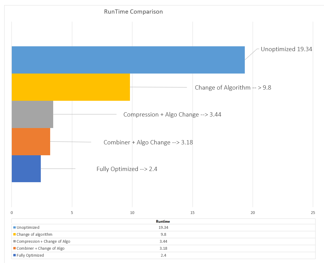
Adding up all the pieces of the puzzle, the cumulative effect of all these 3 optimizations working in tandem greatly reduces the runtime of the code & this is the sort of optimization a developer strives for !! 🙂

These margins will only increase as the size of data increases and so after a really long post, i’ll end this article with one last screenshot and I’ll let the results speak for itself. !!