
In my previous article, I wrote my thoughts on the Paradigm Shift I underwent adapting to the idiosyncrasies of real time systems when compared to batch processing.
Picking up from where I left off, this article focuses on applying all those concepts to build a realtime data enrichment pipeline which performs join & lookup in real time handling massive volume of data. I share my experience along with my rationale behind some of the decisions I made from a programmatic standpoint in building the said system. I will be using the terms Data Enrichment and Joins interchangeably as they both mean the same , atleast from a high level.
I managed to reduce the complexity of the code from O(N2– N) to O(N) reducing the number of queries fired on the database for each key from 12 to 4 for joining across 4 streams (N = 4).
For my sample data set which has around 14,000 transactions / distinct keys ,the total number of search queries fired on the database is reduced from 168,000 to 56,000. Even though ElasticSearch or any distributed document store can easily handle 168K requests, reducing that number to 56K frees up the cluster resources to be used for more meaningful tasks.
- Tools of the Trade
- Bird’s eye view of the problem
- Reality vs Expectation – Existing vs Proposed design
- The actual problem (statement) – Nth time is the charm !!
- Optimized version .. Less is More
- Conclusion
The project is named Fusion which is befitting to its function of joining or fusing multiple data streams produced by disparate systems to one single enriched data model. Those having a penchant for code can head over to the code committed at the below github repo.
https://github.com/kitark06/fusion
One of the most frequented operation on RDBMS systems are Joins. Bringing together and merging data with the goals to enrich it is the primary reason why it is one of the most used operation in an ETL workflow. Now doing this on a bulk of data lying around sitting inside the database seems easy these days as we have grown accustomed to it. You simply use any of the available database engines with a decently crafted schema and the SQL engine takes care of the heavylifting and performs under-the-hood optimization before giving the output.
But when velocity of messages increases to a point where it can’t be realistically processed by RDBMS in the expected time, the big-data ecosystem comes to mind. The data enrichment category which this project currently falls under has myriad business domains different where it can applied.
Some of the Eg include
- Advertising impression tracking
- Augmenting Financial Spend information
- User Click Stream tracking
- Healthcare data enrichment
Tools of the Trade
As this use case screams real time stateful stream processing, my decision to go with Apache Flink as the core processing framework shouldn’t come as a surprise. I chose Flink over Spark Streaming because Flink is purpose built for streaming and it shows !! Its miles ahead of the competition when it comes to the semantics and the general expressivity which the api offers. It also has a excellent stateful operations available, something which will be used to its fullest potential in this project when we optimize it.
It will be supported by Apache Kafka as the ephemeral storage layer which at this point, is really a no-brainer & has become the defacto standard in any streaming system. If you are looking for reasons why Kafka should be used, check this link.
NoSql database ElasticSearch will be assisting kafka as the permanent persistence layer, for storing the final result of the join operation. Also a few intermediate static lookup tables will be stored here.
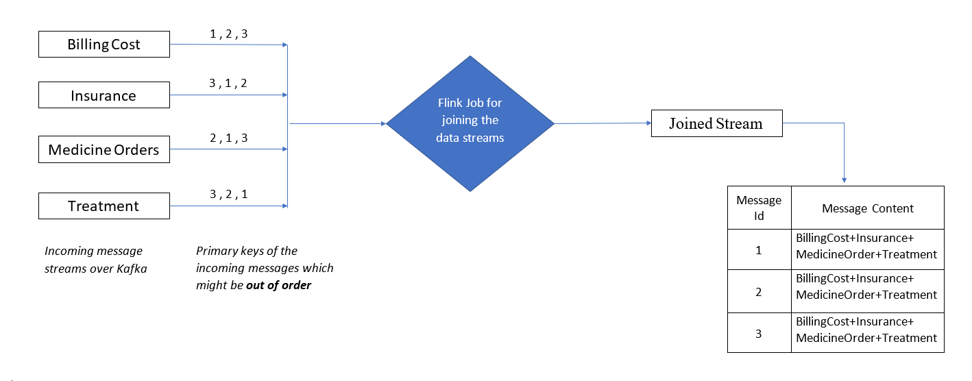
Bird’s eye view of the problem
I will be taking an example where in healthcare data generated from different systems are joined with the goal to derive insights. If this sounds contrived or hypothetical lemme state that this is very similar to a real use case which I designed and implemented for a particular client.
Reality vs Expectation – Existing vs Proposed design
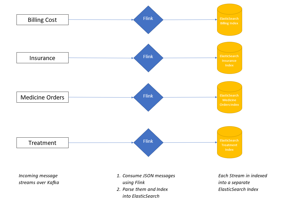
Some parts of the system were already in place when I got the project for development, forcing me to adapt and improvise on the pipeline. The project had a couple of small pipelines running which would take data form Kafka and index it into ElasticSearch which served as a long term permanent storage also providing access to run analytical queries on the documents stored in the indexes.
Existing Setup :
Proposed Design v1 :
We can modify the existing setup to add support for the data enrichment by adding another flink job (in gray) which listens to all 4 topics and joins the messages based on their primary key.
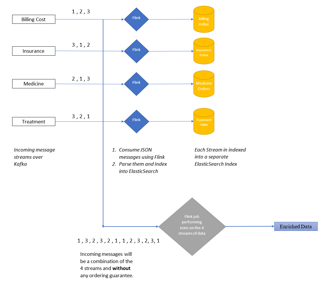
However, there are some practical challenges to this approach
- The messages for a particular key which arrive in the 4 separate streams are produced and inserted into kafka by different components.
- So we have no guarantee about the time duration within which we can say that all of the data for a particular message has arrived.
- Since Kafka is considered more of a temporary storage stream, we can’t reliably store messages in Kafka, as the messages will be deleted after the retention.period elapses.
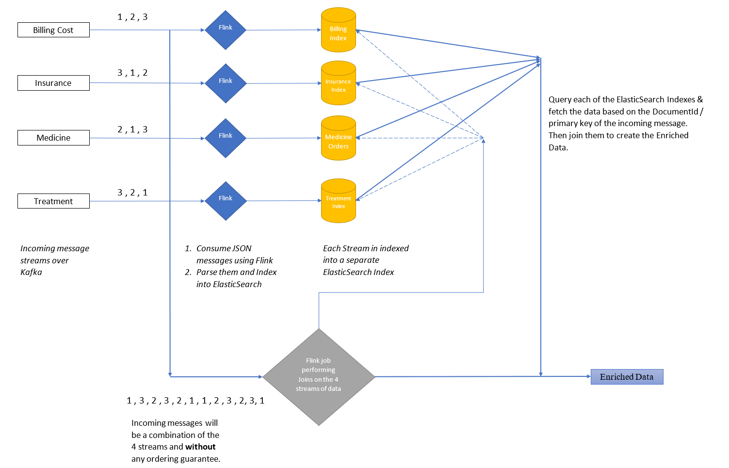
Since the data is already being indexed in ElasticSearch, it makes sense to simply listen to the kafka topics for events and then query Elasticsearch to get the actual data. Implementing this design gives us Proposed Design v2.
Proposed Design v2 :
In this design, we fetch the data from ElasticSearch and only use Kafka as an event stream. This way we have solved the aforementioned limitations of not storing the message on kafka, as by relying on kafka just for the notification or events, we can query ES and get the data.
This way even if the delay between the first and last message belonging to the same key is greater than the retention period of kafka, the message is indexed on ElasticSearch and can be retrieved.
Let me explain. Imagine we have a retention period of 24 hours. That way, messages written will remain on kafka only for one day. If message with Id 1 is written on Kafka, and later the last message is written after 24 hours, the first message will be lost. This is a highly plausible scenario as we cant guarantee when a specific message or a set of messages will arrive in our system. We can work our way around this by setting the retention period of kafka to an unrealistic value so that the messages are practically never removed. But that would cause a humongous disk usage and besides Kafka isn’t meant to be used as a database. Hence we throw that thought out of the window .. No pun intended 🙂
This seems a much better option now, doesn’t it ?? NO .. A simple glance over the solution is enough to draw attention to the real problem which now raises its head !! What we have over here is a naive and brute force way of solving the problem with a Code complexity of O(N2). Let’s break it down to see why.
The actual problem (statement) – Nth time is the charm !!
The matching job receives a stream of incoming messages and has to query each database other than the one which it got the message from. Since the indexing is done from 4 separate Flink Jobs denoted by the blue diamonds, we don’t know which Flink Job has indexed which messages. I mean to say that these Flink jobs are Stateless. So we are left with no option but to blindly fire multiple queries to the ES index in hopes to find the exact moment when all the data used for the join operation will be available.
Based on the assumption that the grey Flink job which does the data enrichment receives its messages in the order (1 , 3 , 2 , 3 , 2 , 1 , 1 , 2 , 3 , 2, 3, 1 ) , lets focus only on messages with ID 1
The flink job goes through each message one by one and sees that the first message it got is [1 , BillingCost]. where 1 is the Id and BillingCost is the message or set of columns. Now since it got the data from BiollingCost Kafka Topic, it wont query that database because it already has that data in the value of the message. For enriching this data, it needs the data from the other 3 Kafka topics for the same messageID 1 , which could be indexed in the ES database. We simply don’t know without firing a search query on ES.
- So for first message which we got [1 , BillingCost]. we fire search queries on the other 3 ES indexes ( Insurance, Medicine & Treatment), all of which will return zero hits because the data for ID 1 hasn’t been encountered.
- For the second message with [1 , Insurance] , we will again query the 3 indexes ( BillingCost, Medicine & Treatment). This time however we will get the BillingCost document but it alone isn’t sufficient for the data enrichment.
- For the third occurance of message with [1 , Medicine ] querying the 3 indexes will fetch us 2 hits from the documents which were indexed before (BillingCost & Insurance)
- Only now when we have the 4th and last piece for the message with ID [1 , Treatment] querying the 3 indexes will return us the desired data from all the indexes and we can proceed with the join operation having all the needed data with us.
I hope now it’s easy to see how the code complexity of the pipeline is
- O(N * (N – 1)) to join all data for a single primary key which gives us O(N2 – N) where N is the number of Kafka Topics or streams across which data is to be joined.
- (N – 1) queries (one for each topic other than the data we already have at the final step) will return the complete data which we can use
- The remaining (N – 1) * (N – 1) queries fired will be wasted as they give us partial results.
Hence in this example where the number of kafka topics is 4, we will be firing
- A total of [4 * (4 – 1)] = 12 queries.
- Out of which [(4-1) * (4-1)] = 9 queries which will be wasted
- & 4 – 1 = 3 will actually give us the desired output
Optimized version .. Less is More
To optimize this design, we need to find a way to query the database at the correct time without bruteforcing it. This can be done by keeping track of all the inserts happening on the database so that we are aware when the final record is indexed in ElasticSearch. What we need is a way to count the inserts happening on the db on a per key level. But since this is a streaming application, the insertion could be done by any one of the streaming application.
Taking help of the stateful computations offered by Flink , we need to create a stateful operator which will keep track of the number of messages flowing in the system. When we encounter a key for the first time, we create a counter for it with value 1. Subsequent encounters of the keys will increment the counter. This counter will work on a partitioned stream. The partitioning the stream will ensure that all the keys of the same value will be sent to the same node. This is taken care by the Flink Framework.
Yes this is similar to the reduce phase in a MapReduce operation. The framework forces us to partition the stream because by sending all the keys to the same node, the counter variable for the key can be cached locally. The state will be maintained locally in the node. This cuts eliminates network and its related problems and challenges from the equation.
Ofcourse, the state is saved in a redundant manner to prevent data loss in case the node processing it dies. This is an ingenious way to cope with the problem of shared state and its called KeyedState.
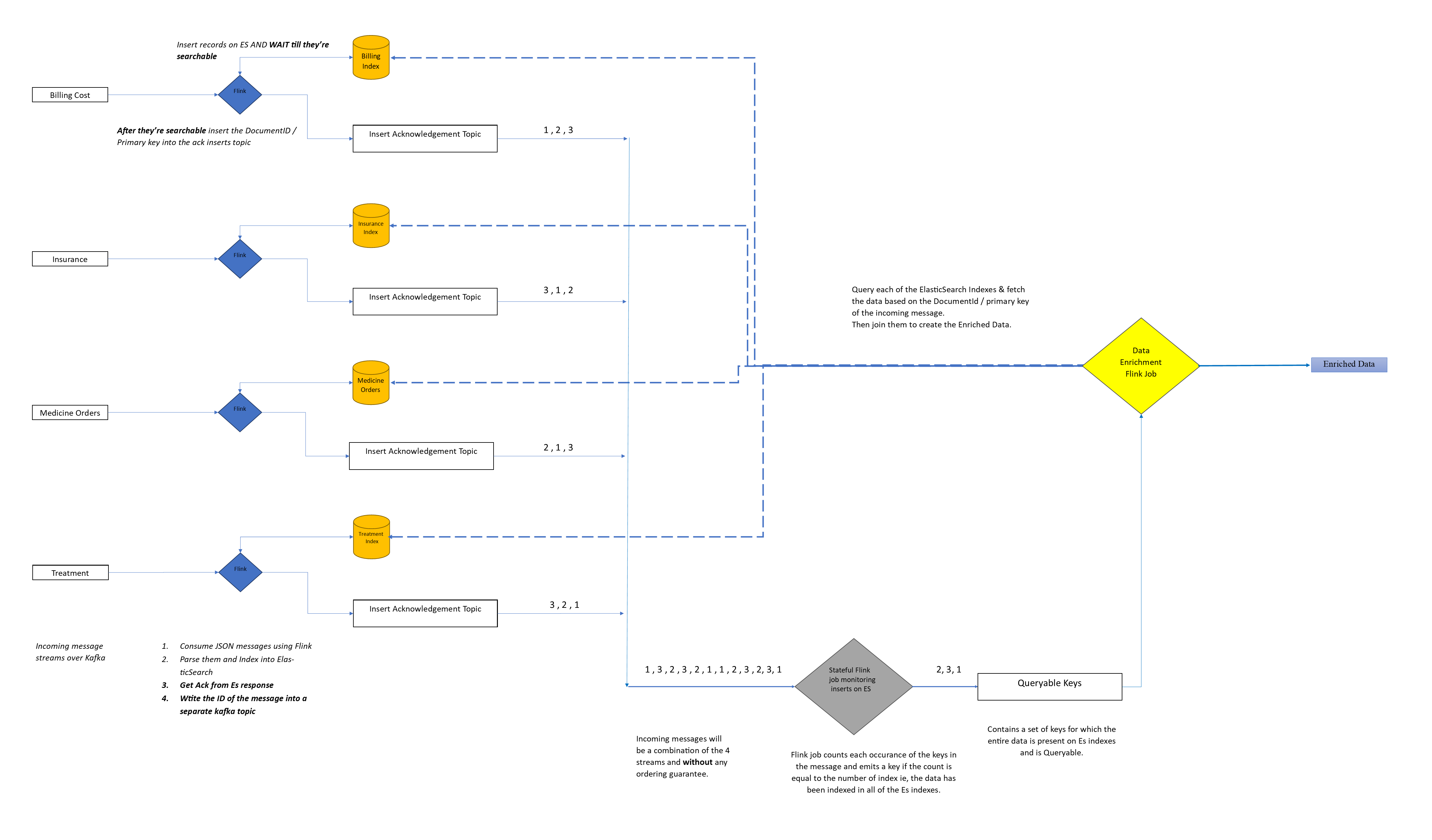
The below pipeline diagram is HUGE and I highly recommend clicking it to enlarge and then view it. The Grey flink job is the stateful mapper responsible for counting and keeping track of the inserts on the database. It listens to the various acknowledgement topics for its counting.
The slight change in this design is the addition of acknowledgement topics. They exist as ElasticSearch is near real time, so there is a slight bit of latency in the time between getting a HTTP status 200 for a successful index and the data actually being searchable. Since this will vary highly based on the load of the cluster, a fixed time based wait is outta the question. Using an additional topic, we have made the operation synchronous in a way that the flink job would wait for the inserts to be indexed AND searchable before sending that message further down the pipeline.
By knowing the precise moment when all the data has been indexed in the databases, it passes the message downstream to the final yellow flink job. The data enrichment job queries all the indexes of ES and now its guaranteed to get all the data which it uses to create the EnrichedDataModel.
About the code.
The project has 2 main classes FusionCore and StreamingCore.
FusionCore is the brains of the project and has the code and the DAG for the pipeline which is responsible for the entire functionality.
StreamingCore is a supporting class with it being responsible for generating a steady stream of input from the input files.
com.kartikiyer.fusion.io.ElasticSearchOperations is the class which has the method performBulkInsert in which requests.setRefreshPolicy(RefreshPolicy.WAIT_UNTIL) causes the method to wait and not return immediately till ES has made the data searchable.
com.kartikiyer.fusion.util.CommonUtilityMethods.getFieldsOfDataModel is responsible for dynamically setting the values in the DataEnrichmentModel using Java Reflection.
Conclusion
By applying a lot of the concepts of Realtime streaming we took what seems to be a simple problem on paper but has lots of new challenges when brought into the bigdata realm. Also we used some of the advance concepts offered by frameworks like Flink to compute stateful processing to reduce the number of queries fired thus optimizing it in the process.
Don’t forget to check the source code of the project at the aforementioned github link at the start of this article. !!
Till next time 🙂
